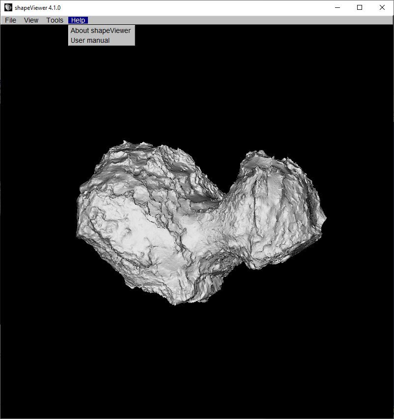
Graphical Interface
shapeViewer aims to be intuitive and ready to use out of the box. The most common functions are accessible directly from the graphical user interface, and via keyboard shortcuts. For instance to simulate observations at a given time: simply click on “View/Set time”. Most menu items have an associated keyboard shortcut, explicitly indicated in the menu entry. For instance, “View/Set Time” uses the letter [T].
When starting the software, a mission is already preconfigured and you can immediately visualize the field of view of different instruments for any epoch covered by the mission scenario.
Main window
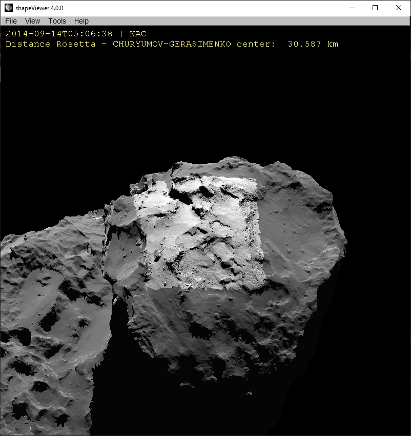
The main window displays a 3D view of the shape(s) currently loaded. Left-click and drag to orient the view, right click to use the current tool. By default, this will give you the coordinates of any point on the surface.
Note
At start, objects are displayed in the following orientation:
Main object:
Z axis (positive, counter-clockwise spin) is pointing UP
X axis (longest, often the prime meridian) is pointing towards the OBSERVER
Secondary objects:
Z axis (positive, counter-clockwise spin) is pointing UP
X axis (longest, often the prime meridian) is pointing towards the MAIN OBJECT
This mimics the most common case of a secondary rotationally locked to its primary (e.g. Earth/Moon), but does not represent the real relative orientation of each object. Use “View/Set Time” to see the real world orientation.
File menu
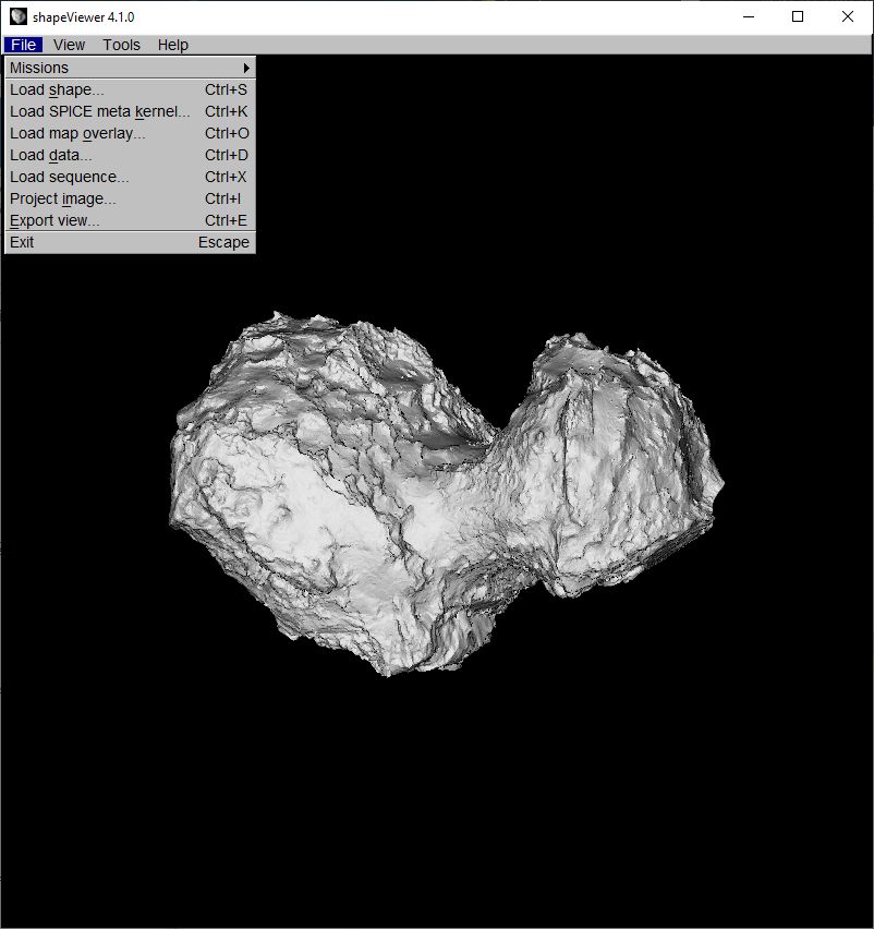
The “File” menu lets you load additional data in the software.
Missions
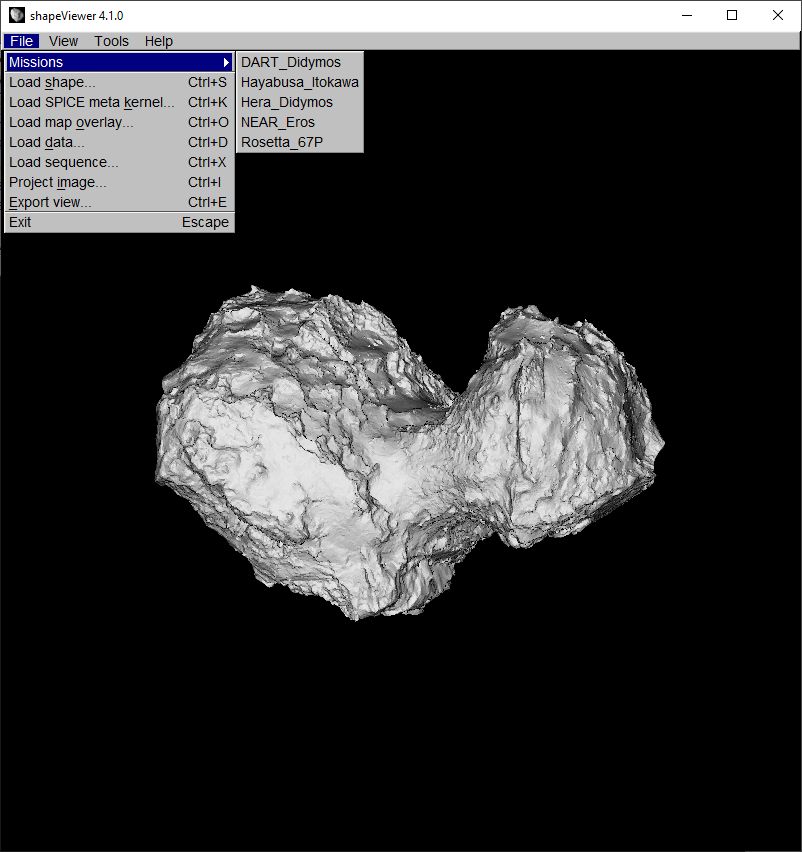
A mission package is a bundle of files that contains everything needed for visualizing a given scenario. This includes shape models, SPICE kernels, instrument details, and so on.
Each package comes with a JSON file which summarizes the relevant information. When starting, shapeViewer will scan the “missions” sub-folder and detect available. When closing the software, it will remember the last mission you were working with.
The structure of a mission package is self-explanatory. To create your own, simply copy an existing JSON file and update it to describe your project.
Shapes
shapeViewer was originally designed to visualize SHAPE files. Although not a common file format in the 3D graphics industry, this has become a standard description for asteroids and comets.
You can find more information on the SHAPE format in the Database of Asteroid Models from Inversion Techniques. Here is a short description:
SHAPE format
3D models are represented as a collection of triangular surface facets. Shape files are a textual representation of those triangles with the following format:
The first line of the file gives the number of vertices and facets,
then follow the x, y, z coordinates of each vertex, one vertex per line
then for each facet the order numbers of facet vertices (anticlockwise seen from outside the body), one facet per line
In addition, shapeViewer also support OBJ and PLY files, with some restrictions:
OBJ files can be of any complexity but only vertices and naked facets are read. Textured facets will not be recognized. Other data is ignored.
PLY format is very versatile, shapeViewer 4 supports headers of the two following types:
Header for PLY Type 1 (Geometry only):
ply
format binary_little_endian 1.0
element vertex ***
property float x
property float y
property float z
element face ***
property list uchar int vertex_indices
end_header
Header for PLY Type 2 (Geometry + vertex color):
ply
format binary_little_endian 1.0
element vertex ***
property float x
property float y
property float z
property uchar red
property uchar green
property uchar blue
element face ***
property list uchar int vertex_indices
end_header
Load SPICE meta kernel
This function lets you replace the current set of SPICE kernels with a new one. In practice, it is recommended to change the default meta kernel in the mission package JSON file.
Load map overlay
Load an image (JPG, PNG) that will be interpreted as a 2D equirectangular map of the current shape model. The image data will be used as a texture for the whole shape.
Load data
User data files can be loaded and displayed. So far, shapeViewer only supports a simple ASCII format to describe the data, similar to the OBJ format for 3D files.
It is foreseen that a new JSON-based data interface will be added in future versions of the software.
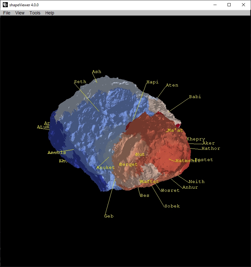
Example of a data file showing region names and borders on comet 67P.
Data is provided as a text file, with one entry per line. Each line starts with the type of data, followed by the relevant information.
Version 4.1.0 supports 4 basic types:
“ms” or “mc” for markers,
“f” for facet data,
“g” for geographic data.
A line starting with any other character will be ignored.
Note
It is possible to mix several types of data in the same file, and/or load multiple files. One could for instance load the thermal map of a given regions, and add coordinate markers to point at areas of interest.
“markers” data:
Displays a line marker and a text label at the given coordinates. Vector information can be provided in spherical (“ms”) or cartesian (“mc”) form.
ms latitude longitude altitude data

| "latitude" and "longitude" in degrees, altitude in km
| "data" is a string, the first space-separated token may be a float number
mc x y z data

| x y z are 3D cartesian coordinates, in km
| "data" is a string, the first space-separated token may be a float number
“facet” data:
Paint the given facets with the given color.
f facet_id R G B data

| "facet_id" is the facet index in the shape model, starting at zero
| "R, G, B" are red-green-blue floats, between 0.0 and 1.0
| "data" is a string, the first space-separated token may be a float number
Line of “geographic” data:
Assign data to the shape model, in areas defined by their central coordinate and angular size. The display will use the current color scheme, which can be changed afterward using the Integrated Console.
g latitude longitude angular_area data

| "latitude, longitude", in degrees, define a point of interest on the shape model
| "angular _area" is the radius of the area that should be considered, in degrees
| "data" is a string, the first space-separated token must be a float number
Note
Loading this type of data can be slow, depending on the number of points and angular size of the regions of interest. Once loaded, it is recommended to export the data to a “facet” file which can be loaded almost instantly in future sessions. See Integrated Console for further information.
Load sequence
Sequences of images can be defined in an JSON file. Once loaded, it will be used to automatically generate simulated images for the given sequence. You must set up what to display (labels, gravity, axes, camera footprints, …) before loading the sequence file.
Each observation in the sequence must define an instrument and a time of observation. An optional texture can be specified and will be projected on the shape.
Example of a sequence.json file:
{
    "sequence": [
        { "camera": "WAC", "time": "2015-01-03T05:35:00", "texture":"WAC_image.jpg" },
        { "camera": "NAC", "time": "2015-01-03T05:35:00" }
    ]
}
Project Image
Load an image corresponding to the current field of view, and project it on the shape. This requires that you have set a time and a camera, the program will remind you to do so if you didn’t.
One projected, the image can be visualized in all views provided by shapeViewer. This means in 3D, but also in the various map projections available in the “View/Projection” menu.
Note: this shape model is shaded with a darker photometric model, to illustrate where the image has been projected. In general, you should use a photmoetric model that matches the data.
Export View
Export the current view to a PNG file in the shapeViewer folder.
This exported view is a PNG using the RGBA color encoding, i.e. the data resolution is limited to 32 bit colors (65536 values) or 8-bit (256) shades of gray. High depth photometric rendering is planned in the near future.
View menu
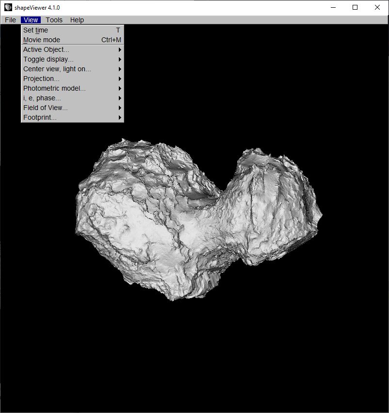
Set time and Movie mode
Probably the most used features. “Set time” let you define an epoch for which you want to simulate what instruments are going to observe. “Movie mode” does the same for the whole mission, and let you select the time displayed simply by clicking on a progress bar at the bottom of the screen (see figure below).
Note that all views are interactive. You can always pause the movie to visualize the shape from another angle than the one displayed, or activate different viewing options interactively.
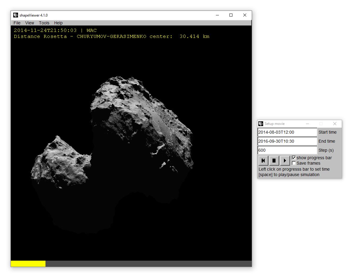
By default the movie mode is configured to display the full mission. You can update the boundaries of the movie in the option windows that appears automatically. Selecting the option “save frames” will export each frame as a PNG file in the “screenshots” folder.
Active Object
The 3D mode displays all objects at once but that is not always possible in other view modes, e.g. map views. In that case, this menu option let you select the object that should be displayed in priority.
Right-clicking an object in 3D view will automatically set that object as active.
Toggle display
shapeViewer can display a lot more information than just a shape model:
axes, coordinate system
elevation
gravity, slopes
surface roughness
direction of the Sun, Observer
incidence, emission, phase
All these options are activated via the “Toggle” menu.
Note
Some information, e.g elevation, is displayed using a color scale. For multiple bodies with very different dimensions (e.g. Didymos and Dimorphos), it is difficult to find a color scale that would fit both objects so shapeViewer will adapt the scale to the current active object. Simply right-click on any object to st it to active
Color scale and limits can be changed using the command line interface.
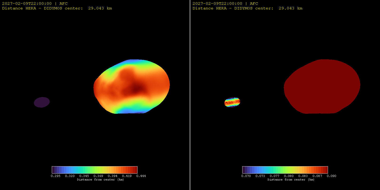
Distance from center of shape in a binary asteroid system. Left: color scale adapted to dimensions of the main object. Right: color scale adapted to dimensions of the secondary.
A note on gravity
shapeViewer provides a model of effective gravitational acceleration (gravity corrected with centrifugal force). The acceleration is calculated for each facet using the model by Cheng+2012, equivalent to the classical Werner&Scheeres+1997 but faster to calculate. shapeViewer assumes a constant density throughout the object.
Results are stored in the “gravity” subfolder. Deleting files in that folder will trigger a prompt for input parameters when trying to display gravity again. Effectively, this allows you to recalculate the acceleration. Note that this is a slow process !
A note on roughness
Surface roughness is defined as the mean angle between a facet nornal vector and its neighbours. It is calculated when the shape is loaded. Details on the algorithm and examples for several small bodies are available in Vincent+2023.
Center view
The items under this submenu will reset the view to preset configurations, by forcing the Sun and Observer position along one of the shape axes (X,Y,Z, -X,-Y,-Z).
Projection
This menu gives you access to several map projections of the active shape.
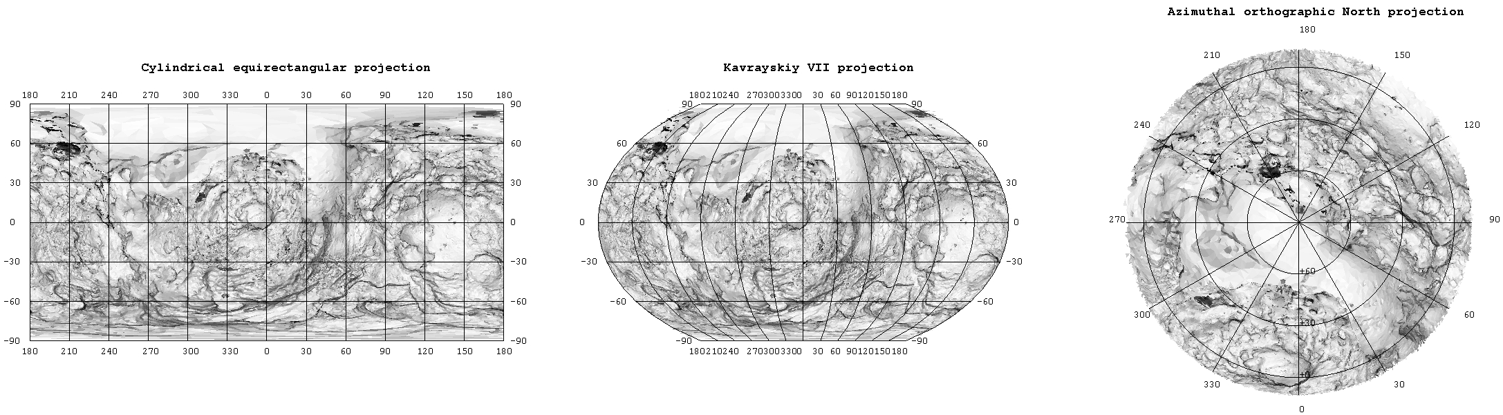
Examples of map projections rendered with shapeViewer
Photometric model
This menu gives you some control on how the shape is being renderd. A few simple photometric models are available in v4 to calculate the reflectance F of the surface:
LAMBERT:         F = u0
LOMMEL_SEELIGER: F = u0/(u0+u)
LUNAR-LAMBERT:   F = u0(1 - L) + 2L * u0/(u0 + u), L in [0,1]
MINNAERT:        F = u0^k * u^(k - 1), k in [0,1]

with u0 = cos(incident angle) and u = cos(emergent angle).
Better model will be included in future versions of the software.
i, e, phase
Display a representation of the incidence, emission, and phase angle at the time of observation. Each angle can be shown individually, or together. In the latter case, angles are encoded in the RGB values of the image (incidence => Red, emission => Green, phase => Blue) with a resolution of 256 values per color.
Field of View
Select the field of view (instrument) to be displayed. The current view will be adjusted to fit this FoV in the frame. This menu is automatically populated from data defined in the mission package.
Footprint
This setting will overlay a box representing an instrument field of view on top of the current scene. It is possible to project the field of view boundaries onto the 3D shape using the command line interface.
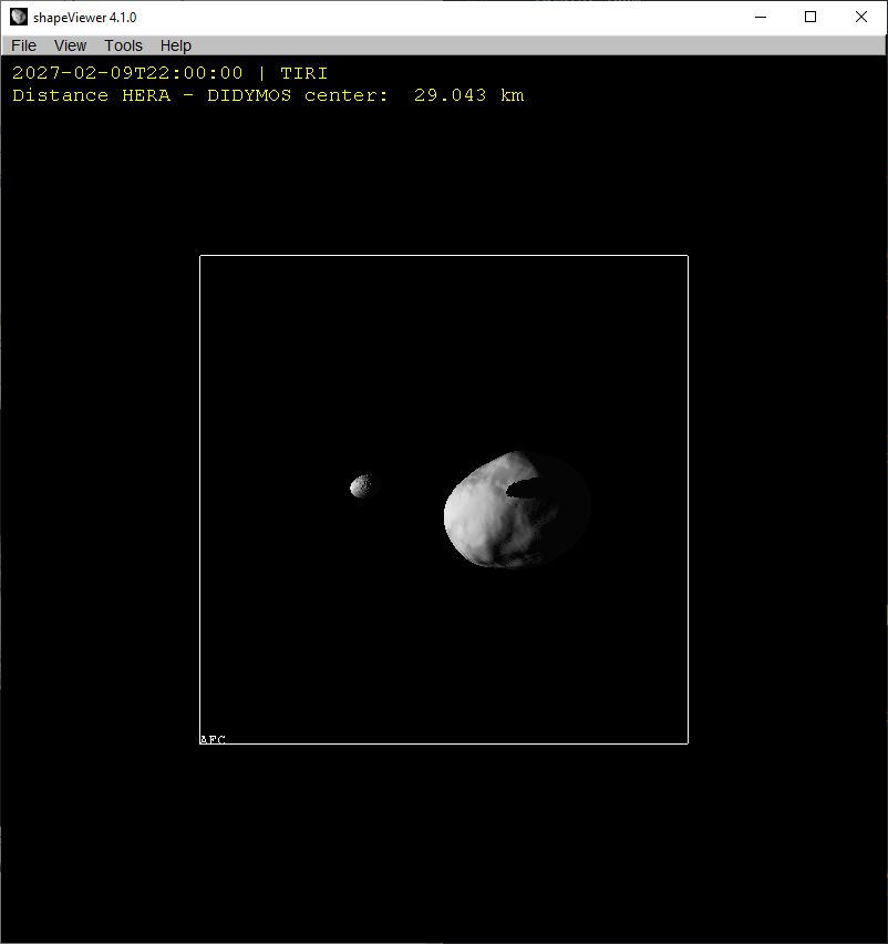
Example of display showing the field of view of Hera’s TIRI instrument as full frame, with the additional footprint of Hera’s AFC instrument.
Tools menu
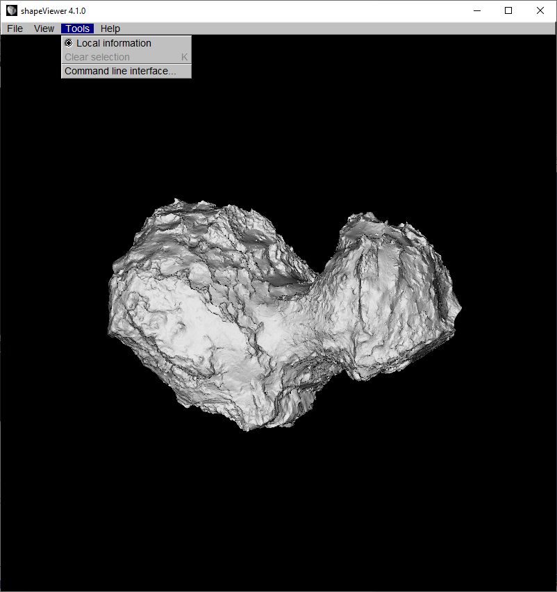
This menu controls what happens when you right-click an object. Most tools are being rewritten and are currently disabled.
Local information
Right-clicking on a shape model gives you access to local information. The amount of information depends on the current selection in the “View menu” and the data available. You can remove this selection by using the menu item “Tools/Clear selection”or the keyboard shortuct [k].
Command line tools
Open a command line interface for advanced options. The command line can also be opened/closed with either the keys [F12] or [=].